Descriptive Statistics
Descriptive statistics allow us to summarize large volumes of raw data into a few meaningful numbers. In Machine Learning, we use these to understand the "center" and the "spread" of our features, which is essential for data cleaning and feature scaling.
1. Measures of Central Tendency
These measures tell us where the "middle" of the data lies.
A. Mean (Average)
The sum of all values divided by the total number of values. It is highly sensitive to outliers.
B. Median
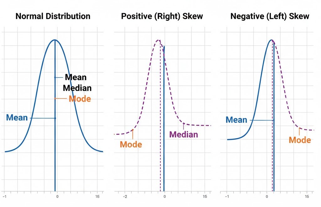
The middle value when the data is sorted. It is robust to outliers, making it better for skewed distributions (like house prices or salaries).
C. Mode
The value that appears most frequently. Useful for categorical data (e.g., finding the most common car color).
2. Measures of Dispersion (Spread)
Knowing the center isn't enough; we need to know how "spread out" the data is.
A. Range
The difference between the maximum and minimum values. Simple, but very sensitive to extreme outliers.
B. Variance ()
The average of the squared differences from the Mean. It measures how far each number in the set is from the mean.
C. Standard Deviation ()
The square root of the variance. It is the most common measure of spread because it is in the same units as the original data.
- Low : Data points are close to the mean.
- High : Data points are spread out over a wide range.
3. Measures of Shape
Beyond center and spread, we look at the symmetry and "peakedness" of the data.
A. Skewness
Measures the asymmetry of the distribution.
- Positive (Right) Skew: Long tail on the right side.
- Negative (Left) Skew: Long tail on the left side.
B. Kurtosis
Measures how "fat" or "thin" the tails of the distribution are compared to a normal distribution. High kurtosis indicates the presence of frequent outliers.
4. Why this matters for ML
- Handling Outliers: If the Mean and Median are far apart, you likely have outliers that could skew your model's training.
- Missing Value Imputation: When filling in missing data, we often choose the Mean (for normal data), Median (for skewed data), or Mode (for categorical data).
- Feature Scaling: Techniques like Z-Score Normalization (Standardization) directly use the Mean and Standard Deviation to rescale features:
Visualizing these numbers is often more intuitive than reading a table. Next, we’ll explore the most important probability distribution in all of science and ML.