PMF vs. PDF

To work with data in Machine Learning, we need a mathematical way to describe how likely different values are to occur. Depending on whether our data is Discrete (countable) or Continuous (measurable), we use either a PMF or a PDF.

1. Probability Mass Function (PMF)

The PMF is used for discrete random variables. It gives the probability that a discrete random variable is exactly equal to some value.

Key Mathematical Properties:

1. Direct Probability: $P(X = x) = f(x)$. The "height" of the bar is the actual probability.
2. Summation: All individual probabilities must sum to 1. $$\sum_{i} P(X = x_i) = 1$$
3. Range: $0 \le P(X = x) \le 1$.

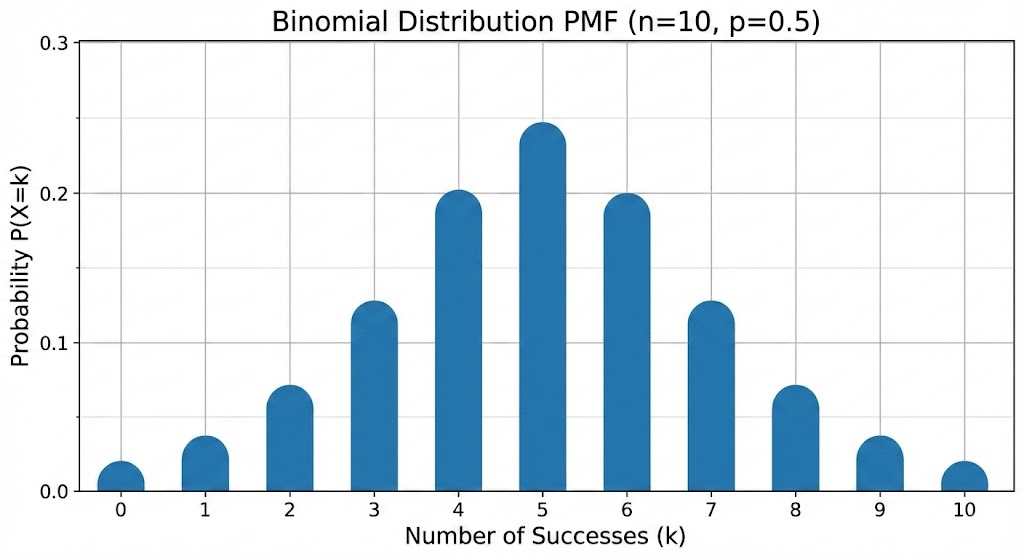
Example: If you roll a fair die, the PMF is $1/6$ for each value $\{1, 2, 3, 4, 5, 6\}$. There is no "1.5" or "2.7"; the probability exists only at specific points.

2. Probability Density Function (PDF)

The PDF is used for continuous random variables. Unlike the PMF, the "height" of a PDF curve does not represent probability; it represents density.

The "Zero Probability" Paradox

In a continuous world (like height or time), the probability of a variable being exactly a specific number (e.g., exactly $175.00000...$ cm) is effectively 0.

Instead, we find the probability over an interval by calculating the area under the curve.

Key Mathematical Properties:

1. Area is Probability: The probability that $X$ falls between $a$ and $b$ is the integral of the PDF: $$P(a \le X \le b) = \int_{a}^{b} f(x) dx$$
2. Total Area: The total area under the entire curve must equal 1. $$\int_{-\infty}^{\infty} f(x) dx = 1$$
3. Density vs. Probability: $f(x)$ can be greater than 1, as long as the total area remains 1.

3. Comparison at a Glance

Feature	PMF (Discrete)	PDF (Continuous)
Variable Type	Countable (Integers)	Measurable (Real Numbers)
Probability at a point	$P(X=x) = \text{Height}$	$P(X=x) = 0$
Probability over range	Sum of heights	Area under the curve (Integral)
Visualization	Bar chart / Stem plot	Smooth curve

---

4. The Bridge: Cumulative Distribution Function (CDF)

The CDF is the "running total" of probability. It tells you the probability that a variable is less than or equal to $x$.

• For PMF: It is a step function (it jumps at every discrete value).
• For PDF: It is a smooth S-shaped curve.

$$F(x) = P(X \le x)$$

5. Why this matters in Machine Learning

1. Likelihood Functions: When training models (like Logistic Regression), we maximize the Likelihood. For discrete labels, this uses the PMF; for continuous targets, it uses the PDF.
2. Anomaly Detection: We often flag a data point as an outlier if its PDF value (density) is below a certain threshold.
3. Generative Models: VAEs and GANs attempt to learn the underlying PDF of a dataset so they can sample new points from high-density regions (creating realistic images or text).

---

Now that you understand how we describe probability at a point or over an area, it's time to meet the most important distribution in all of data science.