Binary search

Binary search is a classic algorithm for finding an element in a sorted array. It repeatedly divides the search interval in half and compares the middle element of the interval to the target value. If the target value matches the middle element, the search is successful. Otherwise, the search continues in the half of the array that may contain the target value.

Why is Binary Search preferred over Linear Search?

1. Time Complexity:

   • Binary Search: O(log n)
   • Linear Search: O(n)

   Binary search divides the search space in half each time, making it much faster for large datasets.

2. Efficiency with Large Datasets:

   • Binary search is efficient for large datasets, requiring around 20 comparisons for a million elements.
   • Linear search would require, on average, 500,000 comparisons for the same dataset.

3. Data Requirements:

   • Binary Search: Requires sorted data.
   • Linear Search: Works with unsorted data but is slower for large datasets.

4. Predictability:

   • Binary search offers consistent performance.
   • Linear search performance varies based on the target element's position.

5. Use Cases:

   • Binary Search: Ideal for static, sorted data with frequent searches (e.g., database indexing, dictionary lookups).
   • Linear Search: Suitable for small datasets or frequently changing data where sorting is impractical.

Algorithm

1. Sort: Ensure the array is sorted in ascending order.
2. Initialize: Set two pointers, low and high, to the beginning and end of the array, respectively.
3. Iterate: While low is less than or equal to high:
   • Calculate the middle index: mid = (low + high) / 2.
   • Compare the middle element with the target value.
   • If the middle element is the target, return the index.
   • If the middle element is greater than the target, search the left half by setting high = mid - 1.
   • If the middle element is less than the target, search the right half by setting low = mid + 1.
4. End: If the target is not found, return an indication (e.g., -1).

Explanation

Recursive Approach

def binary_search_recursive(arr, low, high, target):
    if low > high:
        return -1  # Target not found

    mid = (low + high) // 2

    if arr[mid] == target:
        return mid
    elif arr[mid] > target:
        return binary_search_recursive(arr, low, mid - 1, target)
    else:
        return binary_search_recursive(arr, mid + 1, high, target)

Iterative Approach

def binary_search_iterative(arr, target):
    low = 0
    high = len(arr) - 1

    while low <= high:
        mid = (low + high) // 2

        if arr[mid] == target:
            return mid
        elif arr[mid] > target:
            high = mid - 1
        else:
            low = mid + 1

    return -1  # Target not found

Time Complexity Analysis

1. Recurrence Relation:

   • Each step of the algorithm reduces the search space by half.
   • If T(n) is the time complexity for an array of size n, then: T(n) = T(n/2) + O(1).

2. Master's Theorem:

   • The recurrence relation T(n) = T(n/2) + O(1) fits the form T(n) = aT(n/b) + f(n), where a = 1, b = 2, and f(n) = O(1).
   • According to Master's Theorem: T(n) = O(\log n)

3. Substitution Method:

   • Assume T(n) = O(\log n).
   • Substitute into the recurrence relation: T(n) = T(n/2) + O(1) = O(\log n) + O(1) = O(\log n)

Space Complexity

• The space complexity for the iterative approach is O(1) since it uses a constant amount of extra space.
• The space complexity for the recursive approach is O(\log n) due to the recursive call stack.

Applications

• Searching in a Sorted Array: Efficiently find an element in a sorted array.
• Database Indexing: Quickly locate records in a sorted database.
• Debugging: Find the source of an error in a range of code or data.

Illustration

Initial State

Array: [1, 3, 5, 7, 9, 11, 13, 15, 17, 19]
Target: 7
low = 0, high = 9

Step 1

mid = (0 + 9) // 2 = 4
Array[mid] = 9
9 > 7, so high = mid - 1 = 3

Step 2

low = 0, high = 3
mid = (0 + 3) // 2 = 1
Array[mid] = 3
3 < 7, so low = mid + 1 = 2

Step 3

low = 2, high = 3
mid = (2 + 3) // 2 = 2
Array[mid] = 5
5 < 7, so low = mid + 1 = 3

Step 4

low = 3, high = 3
mid = (3 + 3) // 2 = 3
Array[mid] = 7
7 == 7, target found at index 3

Pictorial Representation

Let us have a pictorial representation of the binary search algorithm to understand it better.

1. The array in which searching is to be performed is:

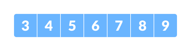
   Initial array

   Let x = 4 be the element to be searched.

2. Set two pointers low and high at the lowest and the highest positions respectively.

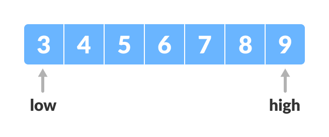
   Setting pointers

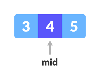
3. Find the middle element mid of the array i.e. arr[(low + high)/2] = 6.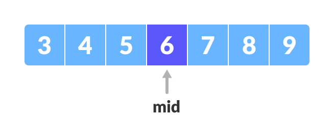

   Mid element

4. If x == mid, then return mid. Else, compare the element to be searched with mid.

5. If x > mid, compare x with the middle element of the elements on the right side of mid. This is done by setting low to low = mid + 1.

6. Else, compare x with the middle element of the elements on the left side of mid. This is done by setting high to high = mid - 1.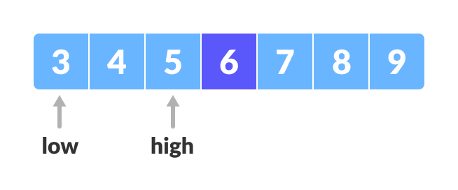

   Finding mid element

7. Repeat steps 3 to 6 until low meets high.

   Mid element

8. x = 4 is found.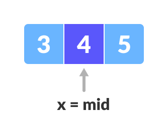

   Found

Binary search is a fundamental algorithm with wide-ranging applications, especially in scenarios requiring fast data retrieval from sorted datasets.